Getting Started
After Installation is complete we try to see if the installation was successful by running the command line interface (CLI) help command:
mpralib --help
It should show the help message with all available commands and options, like this:
Usage: mpralib [OPTIONS] COMMAND [ARGS]...

Command line interface of MPRAlib, a library for MPRA data analysis.

Options:
--help  Show this message and exit.

Commands:
combine        Combine counts with other outputs.
functional     General functionality.
plot           Plotting functions.
validate-file  Validate standardized MPRA reporter formats.
If you see this message, the installation was successful. You can now start using MPRAlib either via the command line interface or as a library within your python code. We recommend to look at the MPRAlib tutorial and the MPRAlib package for using the API or the Command Line Interface for using the command line interface. For a quickstart we provide one CLI and one API example below.
As a quick example we will read the example barcode count file and computing correlation across replicates and plot them. We will do this with the command line interface as well as through the python API.
Preparing Example Data
First we download an example barcode count file to work with using wget from our MPRAlib repository on GitHub:
wget https://github.com/kircherlab/MPRAlib/raw/refs/tags/v0.9.0/resources/barcode_counts.tsv.gz -O example_barcode_counts.tsv.gz
Command Line Interface Example
Now we can use the command line interface to compute correlation across replicates and plot them. We will use the functional compute-correlation command for this. The input is the barcode count file we just downloaded. We want to compute correlation for the activity (log2 normalized RNA over normalized DNA ratio) using --correlation-on activity.
mpralib functional compute-correlation \
--input example_barcode_counts.tsv.gz \
--correlation-on activity
This will compute spearman and pearson correlation across all 3 replicates. The result should look like this:
pearson correlation on Modality.ACTIVITY: [0.967308   0.9596891  0.97339666]
spearman correlation on Modality.ACTIVITY: [0.9279497  0.92303765 0.94871825]
We can also set a minimum number of required barcodes per oligo to remove noisy oligos using --bc-threshold 10 and rerun the command:
mpralib functional compute-correlation \
--input example_barcode_counts.tsv.gz \
--correlation-on activity \
--bc-threshold 10
We should see a slight increase in the correlation values:
pearson correlation on Modality.ACTIVITY: [0.97747856 0.9760033  0.98485214]
spearman correlation on Modality.ACTIVITY: [0.9380415 0.9349714 0.9591882]
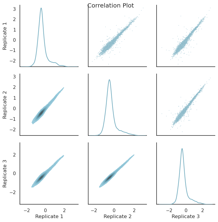
To plot the correlation across replicates use the plot correlation command:
mpralib plot correlation \
--input example_barcode_counts.tsv.gz \
--modality activity \
--output correlation_plot.png
The image example_correlation_plot.png should look similar like this:
Python API Example
We can do the same using the python API. Please start the python console, create a python file, or use a notebook. First we import the library and read in the barcode count file:
import mpralib

# Read in barcode count file
mpra_barcode_data = mpralib.mpradata.MPRABarcodeData.from_file("example_barcode_counts.tsv.gz")
Now we compute the correlation of the oligo data. Because we have the data on a barcode level we first have to aggregate to get to the oligo level. This is simply generating an MPRAOligoLevelData object with the oligo_data getter. Then we can use the correlation method to compute correlation across replicates on the activity level.
# Aggregate to oligo level
mpra_oligo_data = mpra_barcode_data.oligo_data

# Compute correlation on activity
print("🔗 Pairwise Pearson correlation (activity, log2 RNA/DNA ratio):")
activity_corr = mpra_oligo_data.correlation()
print(activity_corr)
The output should be:
🔗 Pairwise Pearson correlation (activity, log2 RNA/DNA ratio):
[[1.         0.967308   0.9596891 ]
 [0.967308   1.         0.97339666]
 [0.9596891  0.97339666 1.        ]]
We can also set a barcode threshold and recompute again:
# Compute correlation on activity with barcode threshold
print("🔗 Pairwise Pearson correlation (activity, log2 RNA/DNA ratio) with barcode threshold 10:")
mpra_oligo_data.barcode_threshold = 10
activity_corr_bc_thresh = mpra_oligo_data.correlation()
print(activity_corr_bc_thresh)
The output should be:
🔗 Pairwise Pearson correlation (activity, log2 RNA/DNA ratio) with barcode threshold 10:
[[1.         0.97747856 0.9760033 ]
 [0.97747856 1.         0.98485214]
 [0.9760033  0.98485214 1.        ]]
Now let’s plot it. To get the same plot as before we have to set the BC threshold back to none (or zero).
# Plot pairwise correlation heatmap for oligo activities
from mpralib.utils.plot import correlation
import matplotlib.pyplot as plt

mpra_oligo_data.barcode_threshold = None
plt = correlation(mpra_oligo_data, mpralib.mpradata.Modality.ACTIVITY)
plt.show()